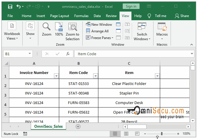
How to Freeze Pane at Columns in Excel worksheet

Sometimes you want to scroll a large worksheet by keeping one or more Columns of a worksheet visible while you scroll columns. For example, you may want to see the first Column of the worksheet while you scroll horizontally to right-side within Excel worksheet. There is a feature in Excel called Freeze Panes to keep some Columns always visible while you scroll horizontally.

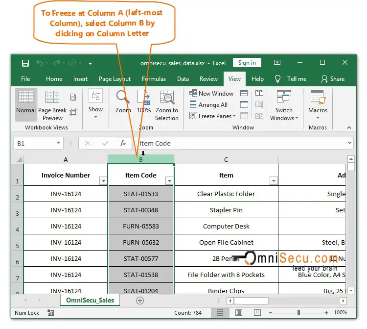
To Freeze Pane vertically at a Column, follow below steps.

Step 1 - Select the right-side Column of the Column which you want to freeze by clicking on its Column Letter, as shown below. In this example, I want to freeze at Column A (left-most column). So I had selected Column B, by clicking on its Column Letter.

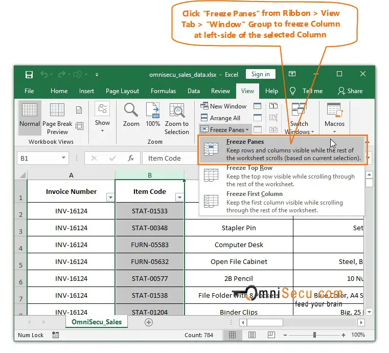
Step 2 - Click "Freeze Panes" menu and then select "Freeze Panes" from Excel Ribbon > "View" Tab > "Window" Group as shown below.

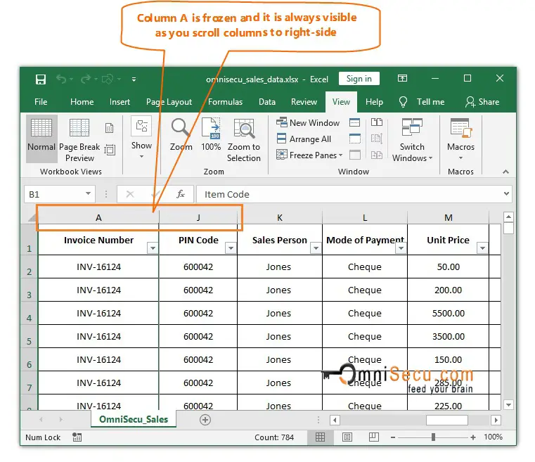
Step 3 - As you can see from below image, Column A is frozen and it is always visible as you scroll to right-side within Excel worksheet.

An animation about how to Freeze an Excel worksheet at a Column is copied below.