How to Freeze Pane at Rows in Excel worksheet

Sometimes you want to scroll a large worksheet by keeping an area of the worksheet always visible while you scroll down. For example, you may want to see the Row Heading of worksheet while you scroll down Excel worksheet. There is a feature in Excel called Freeze Panes to make some Rows of a worksheet always visible while you scroll down Excel worksheet vertically.

To Freeze Pane an Excel worksheet at a Row, follow below steps.

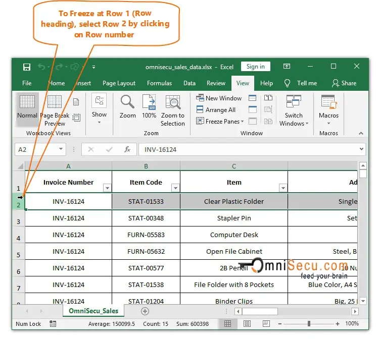
Step 1 - Select the lower Row of the Row which you want to freeze by clicking on its Row number, as shown below. In this example, I want to freeze at Row 1 (top-most Row). So I had selected Row 2, by clicking on its Row number.

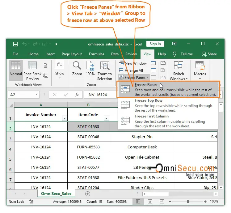
Step 2 - Click "Freeze Panes" Rich menu and then select "Freeze Panes" from Excel Ribbon > "View" Tab > "Window" Group as shown below.

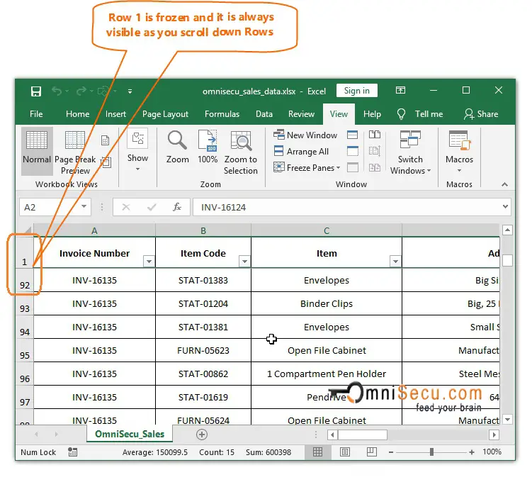
Step 3 - As you can see from below image, Row 1 is frozen and it is always visible as you scroll down Excel worksheet.

An animation about how to Freeze an Excel worksheet at a Row is copied below.